Chapter I Basics

Installation

First you will want to get the R environment. On this website, just choose the right installation for your operating system and you are ready to go.

IDE

IDE (Integrated Development Environment) for R is something nice to have. Because having an IDE can save you lots of time and problems as it has many useful functions. For example, you can directly view the dataset like an excel sheet or run your R script directly from the editor.

Personally I use Rstudio, and I think it is the best, but there are several other options you can choose from such as Rattle and Rgedit.

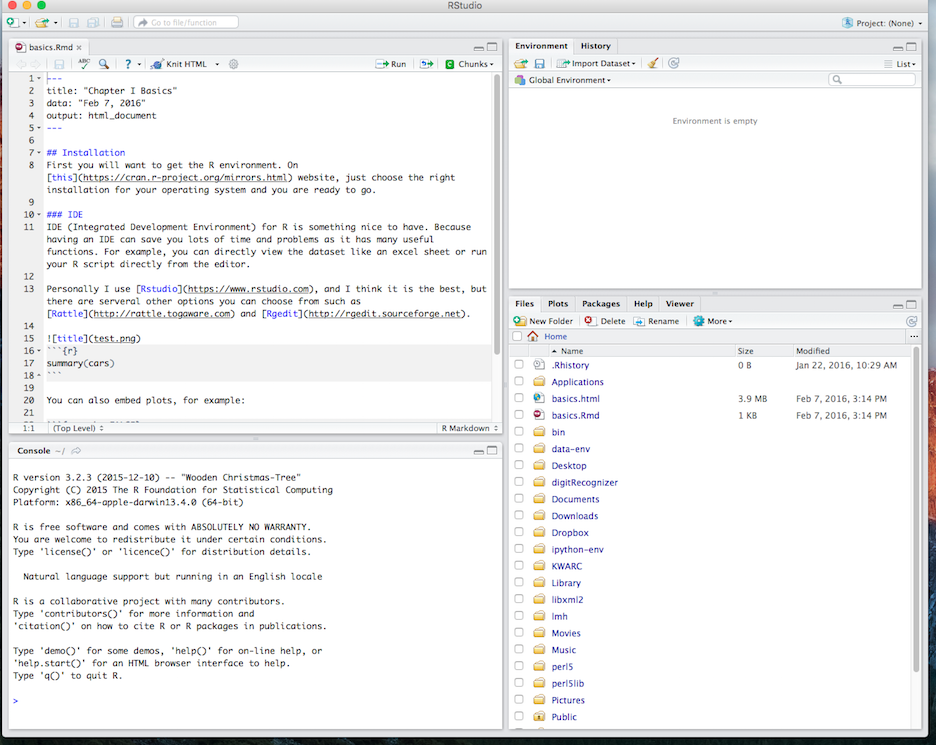
On the top left is the editor for your rScript. On the bottom left is the R Console where you can run the script. On the top right is a list of variables and environment values and on the bottom right is your current directory. If you want to run any particular segment of your R script, you can just highlight that segment and click the run bottom on the top, so that it will be run in your console.

R Basics

Now we can start talking about the R basics and get your hands dirty. I highly suggest you follow along to get yourself more familiar with working with R because R is famous for being unfriendly to newcomers. Even some of my friends who study computer science had a difficult time getting started with R.

Basic Data Types

Before we can make complex analysis using R, we want to know the elements of R just like if we want to cook a dish, we need to know about the ingredients first and then comes to recipe. In the world of R, everything has a type and there are five basic data types:

1. Numeric

x = 3.21
class(x)

## [1] "numeric"

x = 3
class(x)

## [1] "numeric"

We first set x to be 3.21 and the class function tells us which datatype on object is.

2. Integer

x = as.integer(5)
class(x)

## [1] "integer"

x = 3.2
class(x)

## [1] "numeric"

x = as.integer(3.2)
x

## [1] 3

class(x)

## [1] "integer"

For the second 3.2 assignment, because we first cast it into an integer so the decimal part is truncated.

3. Logical

a = TRUE
b = FALSE
a & b

## [1] FALSE

4. Character

my_char = "Hello"
class(my_char)

## [1] "character"

numAsChar = as.character(3.2)
class(numAsChar)

## [1] "character"

After knowing most of the basic datatypes, we can move one step forward.

Dataframe

You may be wondering how those things are going to help me analyze data, and why do we need those datatypes at all? I hope you will find your answers as we progress. You know, having just one variable is boring, can we create a list of them? Yes we can by using vector and later you will find out how to can put multiple vectors together to create a dataframe which is essentially our dataset.

a = 2
b = "second"
c = 3.2
my_vector = c(a, b, c, 3.3)
my_vector

## [1] "2"      "second" "3.2"    "3.3"

We first create a couple variables, and then we put them all into my_vector.

name = c("R", "Python", "Matlab")
yearOfCreation = c(1993, 1989, 1970)
awesomeness = c("Oh yeah", "Ok", "Excuse me?")
df = data.frame(name, yearOfCreation, awesomeness)
df

##     name yearOfCreation awesomeness
## 1      R           1993     Oh yeah
## 2 Python           1989          Ok
## 3 Matlab           1970  Excuse me?

First we have a vector of programming languages, then we have a vector of numeric that entail when each language was created, in the end we give some of our opinions about each language. Hence, we can put those vectors into one big chunk, the dataframe. The layout of the dataframe looks like something we see in data analysis project.

Having learning the R basics and the some essential foundation of R, in the next chapter we can finally start exploring the true power of R by doing some exploratory analysis and find out the correlation between different variables in our data frame.